Cross-validation strategies in QSPR modelling of chemical reactions

• ©  2021 Assima Rakhimbekova

• ©  2021 Ramil Nugmanov

The notebook illustrates how the quantitative structure-property relationship (QRPR) model can be used to predict rate constants of reactions (logK) using bimolecular nucleophilic substitution reactions dataset by Gimadiev et al. as an example. We consider cross-validation of the QRPR models for reactions and show that the conventional k-fold cross-validation procedure gives an ‘optimistically’ biased assessment of prediction performance. To address this issue, we suggest two strategies of model cross-validation, ‘transformation-out’ CV, and ‘solvent-out’ CV. Unlike the conventional k-fold cross-validation approach that does not consider the nature of objects, the proposed procedures provide an unbiased estimation of the predictive performance of the models for novel types of structural transformations in chemical reactions and reactions going under new conditions.

• Loading dataset

• Featurize the reactions using StructureFingerprint linear fingerprints of Condensed Graph of Reactions

• Train and predict QRPR model

  • k-Fold CV

  • Transformation-out CV

  • Solvent-out CV

Loading dataset

from CIMtools.datasets import load_sn2

dataset, Y = load_sn2(return_X_y=True) # dataset - array of reactions,
                                       # Y (what we want to predict) - array of logK

dataset[0]

dataset[0].meta # temperature (K),
                # logK - Y (what we want to predict),
                # additive.1 - solvent,
                # amount.1 - the molar ratio of organic solvent (1.0 for pure solvent)

{'temperature': '298.15',
 'logK': '-4.19',
 'additive.1': 'water',
 'amount.1': '1.0'}

print('Number of reactions = {}'.format(len(dataset)))
print('Number of transformation = {}'.format(len(set(dataset))))

Number of reactions = 4830
Number of transformation = 1352

Featurize the reactions using StructureFingerprint linear fingerprints of Condensed Graph of Reactions

from sklearn.compose import ColumnTransformer
from sklearn.pipeline import Pipeline
from sklearn.preprocessing import StandardScaler, FunctionTransformer
from CIMtools.preprocessing import CGR, EquationTransformer, SolventVectorizer
from CIMtools.preprocessing.conditions_container import DictToConditions, ConditionsToDataFrame
from CIMtools.utils import iter2array
from StructureFingerprint import LinearFingerprint
from numpy import array
from math import sqrt

Helper function for sklearn Pipeline

def extract_meta(x):
    return [y[0].meta for y in x]

Create two Pipelines (see more about Pipeline) for processing structures and conditions.

The following transformers are used:

1. ColumnTransformer assigns specific transformers to each column.

2. EquationTransformer converts the temperature to the required form

3. SolventVectorizer converts the name of the solvent into 13 descriptors. You can specify which of the 13 descriptors to use.

4. If we have additional descriptors, such as the molar ratio of organic solvent, then we can not use transformers, but specify ’passthrough’. For example, for molar ratio of organic solvent it would look like this: (’amount’, ’passthrough’, [’solvent_amount.1′])

5. FunctionTransformer constructs a transformer from an arbitrary callable (see more about FunctionTransformer) in the official site)

6. DictToConditions — helper for mapping dictionary of conditions to conditions objects. It also self-tests, that is, it will check all conditions for validity. DictToConditions implements: temperature, pressure, solvent and molar fraction of solvents. In order to use it, you need to register how each type of condition is indicated in the initial data, and in the case of solvents, you need to indicate a list of the solvent’s names and the names of its molar fraction. Moreover, the names of solvents and molar fractions must be specified in the same order. For example, solvents = [’additive.1′, ’additive.2′] and amounts (means molar fractions) = [’amount.1′, ’amount.2′].

7. ConditionsToDataFrame — a special transformer from CIMtools that turns the list of conditions into a DataFrame, that is, it unpacks the conditions into columns. By default, it will pull out temperature, pressure and solvent.

At the output of the next cell, we get the list of condition objects.

features = ColumnTransformer([('temp', EquationTransformer('1/x'), ['temperature']),
                              ('solvent', SolventVectorizer(), ['solvent.1']),
                              ('amount', 'passthrough', ['solvent_amount.1'])])

conditions = Pipeline([('extract_meta', FunctionTransformer(extract_meta)),
                       ('parse_meta', DictToConditions(solvents=('additive.1',),
                                                       temperature='temperature',
                                                       amounts=('amount.1',))),
                       ('convert', ConditionsToDataFrame()),
                       ('featurize', features)])

The next cell processes the structures of reactions.

graph = Pipeline([('CGR', CGR()),
                  ('convert', FunctionTransformer(iter2array)),
                  ('fingerprint', LinearFingerprint(min_radius=2, max_radius=5, length=1024))])

We combine two Pipelines for processing the structures of reactions and the conditions.

pp = ColumnTransformer([('conditions', conditions, [0]),
                        ('structure', graph, [0])])

We get the descriptors of the CGR of reactions and the conditions

X = pp.fit_transform([[x] for x in dataset])

Train and predict QRPR model

k-Fold CV

from sklearn.model_selection import KFold

cv = KFold(n_splits=5, shuffle=True, random_state=1)

In the cross-validation procedure (we call it as ’Reaction-out’ CV), the initial data set is divided into a given number of subsets, corresponding to the desired number of folds. ’Reaction-out’ CV approach is simply a regular five times repeated five-fold CV. The sizes of test sets in it are almost equal.

from sklearn.ensemble import RandomForestRegressor

Y_pred, Y_true = [], []
for train_index, test_index in cv.split(X):
    x_train = X[train_index]
    x_test = X[test_index]
    y_train = Y[train_index]
    y_test = Y[test_index]
    Y_pred.extend(RandomForestRegressor(random_state=1, n_estimators=500,
                                        n_jobs=-1).fit(x_train, y_train).predict(x_test))
    Y_true.extend(y_test)

Calculate performance metrics (R2, RMSE)

from sklearn.metrics import r2_score, mean_squared_error

print('Q2 = {}'.format(round(r2_score(Y_true, Y_pred),3)))
print('RMSE = {}'.format(round(mean_squared_error(Y_true, Y_pred, squared=False),3)))

Q2 = 0.835
RMSE = 0.474

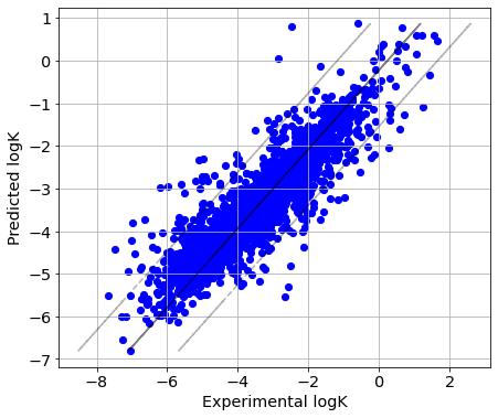
In ‘reaction-out’ CV strategy reactions having the same reactants and products are simultaneously present in both training and test set. Two reactions with very similar conditions can be present in the training and test set, and thus the prediction performance is overoptimistic.

Plot predicted vs experimental logK

import matplotlib.pyplot as plt

plt.rc('font', family='sans-serif')
params = {'legend.fontsize': 'x-large',
          'figure.figsize': (7, 6),
          'axes.labelsize': 'x-large',
          'axes.titlesize':'x-large',
          'xtick.labelsize':'x-large',
          'ytick.labelsize':'x-large'}
plt.rcParams.update(params)

from numpy import arange,array,ones
from scipy import stats

def picture(y_test, y_pred):
    slope, intercept, r_value, p_value, std_err = stats.linregress(y_pred, y_test)
    line = slope * array(y_pred)+intercept

    rmse = sqrt(mean_squared_error(y_test, y_pred))
    fig=plt.figure()
    ax=fig.add_subplot(111, label="1")

    ax.scatter(y_test, y_pred, color="blue", marker='.', s=150)
    ax.set_xlabel("Experimental logK", color='black')
    ax.set_ylabel("Predicted logK", color='black')

    plt.plot(line, y_pred, color='black', alpha=0.5)
    plt.plot(line-3*rmse, y_pred, 'k--', color='black', alpha=0.3)
    plt.plot(line+3*rmse, y_pred, 'k--', color='black', alpha=0.3)

    plt.grid(True)
    plt.rc('xtick')
    plt.rc('ytick')

picture(Y_true, Y_pred)

Transformation-out CV

Helper function for transformation-out and solvent-out CV

def grouper(cgrs, params):
    """
    Helper function for transformation-out and solvent-out CV

    Parameters
    ----------
    cgrs: list
        The list dataset.
    params: list
        What we want to sort by.
        If these are solvents, then we transfer the general
        name of the solvents in the meta data in square brackets.
        For example: ['additive.1']
    Returns
    -------
    groups: tuple
        Tuple of parameters
    """
    groups = []
    for cgr in cgrs:
        group = tuple(cgr.meta[param] for param in params)
        groups.append(group)
    return groups

‘Transformation-out’ CV approach is implemented as a k-fold cross-validation (Figure 1). In the ‘transformation-out’ procedure, all reactions having the same CGR are placed into the same fold (different shapes in Figure 1). The implemented splitting algorithm tries to make the folds approximately equal in size. Therefore, a fold might contain a group of several CGRs (as presented in fold 2, Figure 1). Moreover, the test set contains reactions proceeding in the solvents presented also in the training set, see Figure 1. This allows for avoiding a bias due to the presence of new solvents in the test set. Thus, unique reactions (corresponding to a unique combination of transformation and solvent) are always placed into the training set, see Figure 1. Since in ‘transformation-out’ validation all reactions having the same reactants and products are placed into the same subset (Figure 1), this only shows how well reactions with new reactants and products, i.e. CGRs, are predicted.

from CIMtools.model_selection import TransformationOut

groups = grouper(dataset, ['additive.1'])

cv_tr = TransformationOut(n_splits=5, n_repeats=1, random_state=1, shuffle=True)

Y_true_tr, Y_pred_tr = [], []

for train_index, test_index in cv_tr.split(X=dataset, groups=groups):
    x_train = X[train_index]
    x_test = X[test_index]
    y_train = Y[train_index]
    y_test = Y[test_index]
    Y_true_tr.extend(y_test)
    Y_pred_tr.extend(RandomForestRegressor(random_state=1, n_estimators=500,
                                           n_jobs=-1).fit(x_train, y_train).predict(x_test))

print('Q2 = {}'.format(round(r2_score(Y_true_tr, Y_pred_tr),3)))
print('RMSE = {}'.format(round(mean_squared_error(Y_true_tr, Y_pred_tr, squared=False),3)))

Q2 = 0.563
RMSE = 0.77

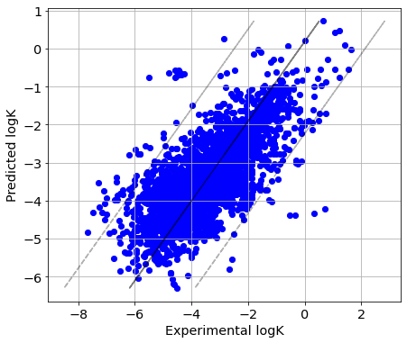
In ‘transformation-out’ CV strategy, all reactions with the same structural transformation are present in either the training or the test sets, but not both simultaneously. Therefore, RMSE values are bigger than for ‘reaction-out’ CV strategy, but they remain on the acceptable levels.

picture(Y_true_tr, Y_pred_tr)

Solvent-out CV

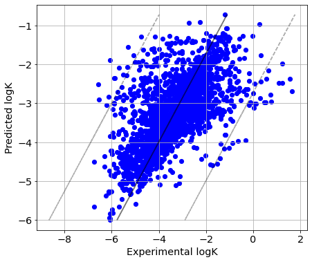
‘Solvent-out’ validation approach is implemented as a leave-one-solvent-out (Figure 1), as the number of solvent types is usually low (less than 50). An additional hurdle to the application of k-fold validation is caused by a great imbalance in the number of reactions corresponding to one solvent. In ‘solvent-out’ validation, all reactions carried out in the same solvent are placed into the same subset which is sequentially used as the test set. Each reaction in the test set should have a counterpart in the training set with the same CGR but proceed in a different solvent. Unique reactions (in this case, reactions measured in a single solvent) are always included in the training set and never used in the test set. This method avoids underestimating of the model performance because such reactions represent new GCR and new solvent for the trained model. It is worth noting that we can group not only by solvents but also following several conditions.

from CIMtools.model_selection import LeaveOneGroupOut

cv_solv = LeaveOneGroupOut()

Y_true_solv, Y_pred_solv = [], []

for train_index, test_index in cv_solv.split(X=dataset, groups=groups): # we group the folds by solvents only
    x_train = X[train_index]
    x_test = X[test_index]
    y_train = Y[train_index]
    y_test = Y[test_index]
    Y_true_solv.extend(y_test)
    Y_pred_solv.extend(RandomForestRegressor(random_state=1, n_estimators=500,
                                             n_jobs=-1).fit(x_train, y_train).predict(x_test))

print('Q2 = {}'.format(round(r2_score(Y_true_solv, Y_pred_solv),3)))
print('RMSE = {}'.format(round(mean_squared_error(Y_true_solv, Y_pred_solv, squared=False),3)))

Q2 = 0.375
RMSE = 0.96

picture(Y_true_solv, Y_pred_solv)